Part 17: Numerical Differentiation for UPSC ISS: Calculus Without Calculators

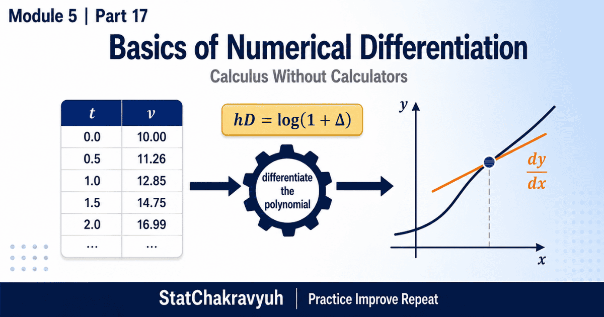
Welcome to Part 17 and the opening of Module 5, updated for the UPSC ISS 2026 to 2027 cycle. With Modules 1 to 4 behind you, interpolation holds no fear. Now we enter the highest weightage block of the Numerical Analysis unit: calculus without calculators, beginning with Numerical Differentiation.

Numerical differentiation evaluates the derivative of a function at a particular value of the independent variable when only a set of discrete values of the function is given. The method: replace the unknown function by an interpolating polynomial, then differentiate the polynomial. At the starting point, the formula is $\left(\dfrac{dy}{dx}\right)_{x_0} = \dfrac{1}{h}\left[\Delta y_0 – \dfrac{1}{2}\Delta^2 y_0 + \dfrac{1}{3}\Delta^3 y_0 – \dots\right]$, the series form of $hD = \log(1 + \Delta)$.

The stakes are at their peak here. Statistics Paper 1 gives 80 questions worth 200 marks in 2 hours, 2.5 marks per correct answer and about 0.83 deducted per wrong one. Numerical differentiation and integration together form the single largest question block of the roughly 20 Numerical Analysis questions, which is why Module 5 is the biggest scoring module of the series.

This post is Part 17 of the Numerical Calculus Guide (Module 5), inside our UPSC ISS Numerical Analysis Complete Guide. New to the exam? Start at the UPSC ISS hub.

The Story of Rakesh and the Rocket Launch

Rakesh, a young ISS officer deputed to ISRO, watches the telemetry system record the rocket’s velocity at equal 10 second intervals:

$t$ (seconds): 0, 10, 20, 30, 40 $v$ (metres per second): 0, 200, 600, 1200, 2000

The Mission Director shouts: what was the exact acceleration at the moment of lift off, $t = 0$?

Acceleration is the derivative of velocity, but Rakesh has no algebraic equation like $v = 3t^2$ to differentiate. He has only a table of numbers. His answer: fit a Newton Gregory Forward polynomial, since $t = 0$ sits at the beginning of the table, and differentiate the formula itself.

The Two Step Method and the Golden Rule

Step 1, approximate: replace the unknown continuous function with a suitable interpolating polynomial. Step 2, differentiate: differentiate that polynomial as many times as needed.

The golden rule of formula choice, exactly parallel to interpolation: near the beginning of the table use Newton Gregory Forward; near the end use Newton Gregory Backward; near the middle use Stirling or Bessel; for unequal intervals differentiate Newton’s Divided Difference or Lagrange’s polynomial.

The Magic Formulas at $x = x_0$

At the exact starting point, $u = \dfrac{x – x_0}{h} = 0$, and the differentiated forward formula collapses beautifully:$$\left(\frac{dy}{dx}\right)_{x = x_0} = \frac{1}{h}\left[\Delta y_0 – \frac{1}{2}\Delta^2 y_0 + \frac{1}{3}\Delta^3 y_0 – \frac{1}{4}\Delta^4 y_0 + \dots\right]$$

The second derivative at the same point:$$\left(\frac{d^2y}{dx^2}\right)_{x = x_0} = \frac{1}{h^2}\left[\Delta^2 y_0 – \Delta^3 y_0 + \frac{11}{12}\Delta^4 y_0 – \dots\right]$$

StatChakravyuh Pro Tips

1. The log E shortcut, heavily tested. No memorization needed. From Part 2, $E = e^{hD}$, so $hD = \log E = \log(1 + \Delta)$. Expand the logarithm: $hD = \Delta – \dfrac{\Delta^2}{2} + \dfrac{\Delta^3}{3} – \dots$ Divide by $h$ and the first derivative formula appears with zero calculus.
2. Maxima and minima of tabulated data. Write the first derivative expression in terms of $u$ from the appropriate interpolation formula, equate it to zero, solve for the critical $u$, and substitute back. Continuous calculus logic, discrete data.
3. Sign discipline. The series alternates strictly: plus, minus, plus, minus. Half the wrong options are sign slips at the second term.

Solved Example Masterclass

Question: $y = f(x)$ is tabulated as $x$: 0, 1, 2, 3 and $y$: 1, 2, 11, 34. Find $\dfrac{dy}{dx}$​ at $x = 0$.

Step 1: Parameters. The point $x = 0$ sits at the beginning, so use the forward shortcut with $h = 1$.

Step 2: Leading differences by mental math. Entries 1, 2, 11, 34. First differences: 1, 9, 23, so $\Delta y_0 = 1$. Second: 8, 14, so $\Delta^2 y_0 = 8$. Third: 6, so $\Delta^3 y_0 = 6$.

Step 3: Apply the formula.$$\frac{dy}{dx} = \frac{1}{1}\left[1 – \frac{1}{2}(8) + \frac{1}{3}(6)\right] = 1 – 4 + 2 = -1$$

Final Answer: $-1$. Cross check: the constant third differences reveal the cubic $f(x) = x^3 + x^2 – x + 1$, whose derivative $3x^2 + 2x – 1$ indeed equals $-1$ at zero. A calculus problem finished with additions and subtractions.

Common Traps to Avoid

Trap 1: Using the forward derivative shortcut for a point at the end of the table. The backward formula owns that territory.

Trap 2: Dropping the $\dfrac{1}{h}$​ factor when $h \neq 1$. The derivative scales with the interval.

Trap 3: Forgetting the alternating signs. Write the coefficient row $1, -\tfrac{1}{2}, +\tfrac{1}{3}, -\tfrac{1}{4}$​ before substituting numbers.

Frequently Asked Questions

Take the Next Step with StatChakravyuh

Join the Free UPSC ISS WhatsApp Community. Every part of this series, plus the Module 5 Practice PDF with 60 MCQs, is delivered there first. 👉 Join the WhatsApp Community now

Enroll in the Free UPSC ISS Course. Structured lessons and practice sets built on the Practice Improve Repeat system, at zero cost. 👉 Enroll in the Free Course

Coming up in Part 18: we flip differentiation on its head. Numerical Integration begins with the mother of all rules, the General Quadrature Formula.