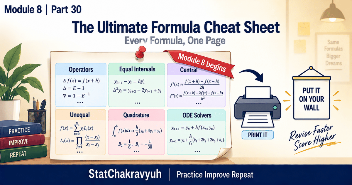
Part 30: UPSC ISS Numerical Analysis Formula Sheet: The Ultimate Cheat Sheet

Welcome to Part 30 and the opening of Module 8, the Last Minute Revision module, updated for the UPSC ISS 2026 to 2027 cycle. Twenty nine parts of theory sit behind you. With the exam approaching, flipping through hundreds of pages is no longer an option; you need one centralized, rapid fire memory aid. This is it: the Ultimate Formula Cheat Sheet, containing only the pure formulas and the golden rules of when to use them. Bookmark this page, print it, and pin it above your desk.

The exam context one final time: 80 questions worth 200 marks in 2 hours, 2.5 marks per correct answer, about 0.83 deducted per wrong one, close to 20 questions from Numerical Analysis, roughly 90 seconds per question, no calculator.

This post is Part 30 of the Last Minute Revision Guide (Module 8), inside our UPSC ISS Numerical Analysis Complete Guide. Full roadmap at the UPSC ISS hub.

1. Operator Algebra Magic Relations

The building blocks from Module 1. Know these and you can derive almost anything in the hall.

Shift, forward, and backward: $E = 1 + \Delta$, $\nabla = 1 – E^{-1}$, and the classic identity $\Delta – \nabla = \Delta\nabla$.

The calculus bridge: $E = e^{hD}$, hence $hD = \log(1 + \Delta) = -\log(1 – \nabla)$.

Central operators: $\delta = E^{1/2} – E^{-1/2}$ and $\mu = \tfrac{1}{2}\left(E^{1/2} + E^{-1/2}\right)$, with the tested identity $\mu^2 = 1 + \tfrac{\delta^2}{4}$.

Differences of zero: $\Delta^n 0^m = 0$ whenever $n > m$, and $\Delta^n 0^n = n!$.

2. Interpolation for Equal Intervals

From Module 2. Use when the gap $h$ is constant.

Newton Gregory Forward, strictly for targets near the beginning of the table:$$f(a + hu) = f(a) + u\,\Delta f(a) + \frac{u(u-1)}{2!}\Delta^2 f(a) + \frac{u(u-1)(u-2)}{3!}\Delta^3 f(a) + \dots$$

Newton Gregory Backward, strictly for targets near the end:$$f(a + nh + uh) = f(a + nh) + u\,\nabla f(a + nh) + \frac{u(u+1)}{2!}\nabla^2 f(a + nh) + \dots$$

3. Central Difference Interpolation

From Module 3. Rapid convergence near the middle of the table.

Stirling’s formula, for $-\tfrac{1}{4} < u < \tfrac{1}{4}$​:$$y_u = y_0 + u\left[\frac{\Delta y_{-1} + \Delta y_0}{2}\right] + \frac{u^2}{2!}\Delta^2 y_{-1} + \frac{u(u^2 – 1)}{3!}\left[\frac{\Delta^3 y_{-2} + \Delta^3 y_{-1}}{2}\right] + \dots$$

Bessel’s formula, for $\tfrac{1}{4} < u < \tfrac{3}{4}$​, with all odd differences vanishing at $u = \tfrac{1}{2}$​:$$y_u = \frac{y_0 + y_1}{2} + \left(u – \frac{1}{2}\right)\Delta y_0 + \frac{u(u-1)}{2!}\left[\frac{\Delta^2 y_{-1} + \Delta^2 y_0}{2}\right] + \dots$$

4. Interpolation for Unequal Intervals

From Module 4. For scattered data.

Newton’s Divided Difference formula, with the equal interval bridge $f(x_0, \dots, x_n) = \dfrac{\Delta^n f(x_0)}{n!\,h^n}$:$$f(x) = f(x_0) + (x – x_0)f(x_0, x_1) + (x – x_0)(x – x_1)f(x_0, x_1, x_2) + \dots$$

Lagrange’s formula, table free, with $\sum L_i(x) = 1$ always, and $x$ and $y$ interchangeable for inverse interpolation:$$f(x) = \frac{(x – x_1)(x – x_2)\cdots}{(x_0 – x_1)(x_0 – x_2)\cdots}f(x_0) + \frac{(x – x_0)(x – x_2)\cdots}{(x_1 – x_0)(x_1 – x_2)\cdots}f(x_1) + \dots$$

5. Numerical Integration (Quadrature)

From Module 5, all children of the Newton Cotes mother formula.

Trapezoidal Rule ($n = 1$), any number of intervals, exact for degree 1:$$I = \frac{h}{2}\left[(y_0 + y_n) + 2(y_1 + y_2 + \dots + y_{n-1})\right]$$

Simpson’s 1/3 Rule ($n = 2$), even intervals required:$$I = \frac{h}{3}\left[(y_0 + y_n) + 4(y_1 + y_3 + \dots) + 2(y_2 + y_4 + \dots)\right]$$

Simpson’s 3/8 Rule ($n = 3$), intervals in multiples of 3:$$I = \frac{3h}{8}\left[(y_0 + y_n) + 3(y_1 + y_2 + y_4 + \dots) + 2(y_3 + y_6 + \dots)\right]$$

Weddle’s Rule ($n = 6$), intervals in multiples of 6, at least 7 points:$$I = \frac{3h}{10}\left[y_0 + 5y_1 + y_2 + 6y_3 + y_4 + 5y_5 + y_6\right] \text{ per block}$$

In the composite form across 12 or more intervals, the junction ordinate shared by two blocks carries weight 2.

6. Difference Equations and ODE Solvers

From Module 6 and Module 7.

First order homogeneous difference equation: $u_{x+1} – a\,u_x = 0$ solves to $u_x = c\,a^x$.

Particular Integral shortcut: for $f(E)u_x = a^x$, $\text{PI} = \dfrac{a^x}{f(a)}$​ when $f(a) \neq 0$.

Euler’s Method (RK1): $y_{n+1} = y_n + h\,f(x_n, y_n)$.

Modified Euler (RK2): Predictor $y_1^{(0)} = y_0 + h\,f(x_0, y_0)$; Corrector $y_1^{(n+1)} = y_0 + \tfrac{h}{2}\left[f(x_0, y_0) + f(x_1, y_1^{(n)})\right]$.

Runge Kutta 4: $y_1 = y_0 + \tfrac{1}{6}\left(k_1 + 2k_2 + 2k_3 + k_4\right)$.

Frequently Asked Questions

Take the Next Step with StatChakravyuh

Join the Free UPSC ISS WhatsApp Community. The Module 8 PDF, carrying this sheet in printable A4 form plus the Top 100 PYQ mix, releases in the community. 👉 Join the WhatsApp Community now

Enroll in the Free UPSC ISS Course. Structured lessons and practice sets on the Practice Improve Repeat system, at zero cost. 👉 Enroll in the Free Course

Coming up in Part 31: the ultimate lifesaver, the Exactness and Error Bounds Master Tables, dissecting local versus global errors and polynomial degrees side by side.