Part 13: Divided Differences for UPSC ISS: Definition, Symmetry, and Exam Tricks

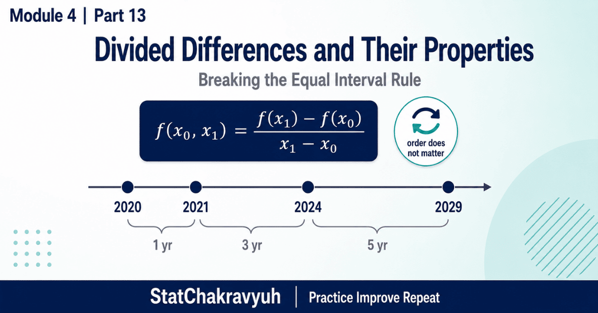
Welcome to Part 13 and the opening of Module 4, updated for the UPSC ISS 2026 to 2027 cycle. In Modules 1 to 3 we lived in a perfect world where every formula, from Newton Gregory to Stirling and Bessel, demanded equally spaced arguments. Real data is rarely that polite. When the intervals turn unequal, every earlier formula collapses, and we enter the world of Divided Differences, a topic the official syllabus names explicitly as “divided differences and their properties”.

The first divided difference is $f(x_0, x_1) = \dfrac{f(x_1) – f(x_0)}{x_1 – x_0}$​, and higher orders follow the recursion $f(x_0, \dots, x_n) = \dfrac{f(x_1, \dots, x_n) – f(x_0, \dots, x_{n-1})}{x_n – x_0}$​. Their defining superpower: they are symmetric functions of their arguments.

The exam context: 80 questions worth 200 marks in 2 hours, 2.5 marks per correct answer, about 0.83 deducted per wrong one, with close to 20 questions from Numerical Analysis. This module’s questions are mostly theory and property based, which makes them the fastest marks on the paper for a prepared aspirant.

This post is Part 13 of the Unequal Intervals and Inverse Interpolation Guide (Module 4), inside our UPSC ISS Numerical Analysis Complete Guide. New to the exam? Start at the UPSC ISS hub.

The Story of Arjun and the Broken Sensor

Arjun, an ISS officer at the Central Ground Water Board, tracks the ground water level of a drought prone district through an automatic yearly sensor. Power failures ruined the schedule: the machine recorded data only for 2020, 2021, 2024, and 2029. The gaps are 1 year, then 3 years, then 5 years. Completely unequal.

When the minister asks Arjun to estimate the level for 2025, Newton Gregory and Stirling are useless, since both demand a constant $h$. Arjun instead builds a divided difference table, which accounts for the actual change in $x$ at every single step.

What Are Divided Differences

When the arguments $x_0, x_1, \dots, x_n$ are not necessarily equally spaced, we define differences by dividing the change in the entry by the actual change in the argument.

First divided difference for two arguments:$$f(x_0, x_1) = \frac{f(x_1) – f(x_0)}{x_1 – x_0}$$

Second divided difference for three arguments, built from the first ones:$$f(x_0, x_1, x_2) = \frac{f(x_1, x_2) – f(x_0, x_1)}{x_2 – x_0}$$

General nn nth divided difference for $n + 1$ arguments:$$f(x_0, x_1, \dots, x_n) = \frac{f(x_1, \dots, x_n) – f(x_0, \dots, x_{n-1})}{x_n – x_0}$$

Note the denominator of each stage: the extreme arguments of that stage, not the adjacent ones. This detail is a favourite trap.

The Superpower: The Symmetric Property

Theorem. Divided differences are symmetric functions of their arguments. The value of any divided difference is independent of the order of the arguments.

In simple words: shuffle the $x$ values however you like, and the divided difference stays exactly the same. For example, $f(x_0, x_1) = f(x_1, x_0)$ and $f(x_0, x_1, x_2) = f(x_2, x_1, x_0) = f(x_1, x_0, x_2)$.

The reason is visible in the expanded symmetric form of the first difference:$$f(x_0, x_1) = \frac{f(x_0)}{x_0 – x_1} + \frac{f(x_1)}{x_1 – x_0}$$

Swapping $x_0$​ and $x_1$​ leaves the sum untouched. Even an upside down table gives the identical highest order difference.

StatChakravyuh Pro Tips

1. The constant polynomial trick. The $n$th divided difference of a polynomial of degree $n$ is a strict constant. For $f(x) = a x^n$, that constant is simply the leading coefficient $a$, and every higher order divided difference is zero. This one rule dissolves the scariest looking questions.
2. The determinant quotient. A repeated theory point: the $n$th divided difference can be expressed as the quotient of two determinants, each of order $n + 1$.
3. The bridge to ordinary differences. For equally spaced data with interval $h$:

$$f(x_0, x_1, \dots, x_n) = \frac{\Delta^n f(x_0)}{n!\, h^n}$$

So divided differences are not a separate universe; they contain the ordinary differences of Module 1 as a special case.

Solved PYQ Masterclass

PYQ pattern (leading coefficient type, the classic trap of this module): What is the third order divided difference of $f(x) = x^3$ for the scattered arguments 2, 4, 9, and 10?

(a) 1 (b) 2 (c) 3 (d) 4

The long way, which is the trap. Compute $f(2) = 8$, $f(4) = 64$, $f(9) = 729$, $f(10) = 1000$, then grind first differences like $\dfrac{64 – 8}{4 – 2} = 28$ and $\dfrac{729 – 64}{9 – 4} = 133$, then second and third differences with three digit divisions and no calculator. Five minutes and one slip away from negative marking.

The StatChakravyuh way, 10 seconds. The function is a polynomial of degree 3, the question asks for the third order divided difference, and the rule says the answer is the leading coefficient. For $x^3$ the leading coefficient is 1.

Final Answer: (a) 1, solved by reading the question.

Quick warm up: for $f(x) = x^2$ with arguments 1 and 3, the first divided difference is $\dfrac{9 – 1}{3 – 1} = 4$, one mental division.

Common Traps to Avoid

Trap 1: Using adjacent arguments in the denominator of higher differences. The general recursion divides by the extreme arguments $x_n – x_0$ of that stage.

Trap 2: Grinding a full table when the function is a polynomial and the question asks for the difference of matching order. The leading coefficient rule answers instantly.

Trap 3: Assuming order matters. Symmetry guarantees it does not, and options exploiting a shuffled order are free marks for those who know the property.

Frequently Asked Questions

Take the Next Step with StatChakravyuh

Join the Free UPSC ISS WhatsApp Community. Every part of this series, plus the Module 4 Practice PDF with 40 MCQs, is delivered there first. 👉 Join the WhatsApp Community now

Enroll in the Free UPSC ISS Course. Structured lessons and practice sets built on the Practice Improve Repeat system, at zero cost. 👉 Enroll in the Free Course

Coming up in Part 14: we assemble these divided differences into the mighty Newton’s Divided Difference Formula, the universal interpolator of the syllabus.