Part 25: Euler Maclaurin Summation Formula for UPSC ISS: The Discrete Continuous Bridge

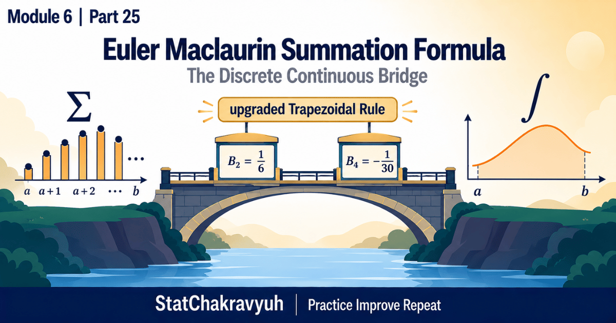
Welcome to Part 25, the grand finale of Module 6, updated for the UPSC ISS 2026 to 2027 cycle. Parts 23 and 24 lived in the purely discrete world, while Module 5 lived in the continuous one. Today the two worlds shake hands across the most elegant bridge in the syllabus: the Euler Maclaurin Summation Formula.

The formula connects a discrete sum of functional values with a continuous definite integral. Its first bracket is exactly the Trapezoidal Rule, upgraded by correction terms that use only odd order derivatives at the two boundary points, with coefficients born from the Bernoulli numbers $B_2 = \tfrac{1}{6}$ and $B_4 = -\tfrac{1}{30}$​.

Exam context: 80 questions, 200 marks, 2 hours, 2.5 marks per question, about 0.83 deducted per wrong answer. Euler Maclaurin questions are almost always structural one liners, which makes this short part one of the best marks per minute investments of the entire series.

This post is Part 25 of the Summation of Series and Difference Equations Guide (Module 6), inside our UPSC ISS Numerical Analysis Complete Guide. Roadmap at the UPSC ISS hub.

The Story of Priya and the Massive Series

Priya, an ISS officer in the Department of Economic Affairs, is building a depreciation model that requires the exact sum $S = 1^4 + 2^4 + 3^4 + \dots + 100^4$. Her intern attacks it with algebraic expansion formulas and drowns in arithmetic.

Priya remembers her training: adding discrete numbers is mathematically close to finding the continuous area under a curve. She applies the Euler Maclaurin formula, integrates $\int x^4\,dx$ instead of adding 100 terms, attaches a few boundary derivative corrections, and lands the exact total in 3 lines.

The Core Concept: An Upgraded Trapezoidal Rule

The formula’s derivation reveals its identity: it is a highly upgraded Trapezoidal Rule. The plain rule gives an approximate area; Euler Maclaurin appends derivative based correction terms that sharpen the answer dramatically.

The master formula, integration form, over $n$ sub intervals of width $h$:$$\int_{x_0}^{x_n} f(x)\,dx = h\left[\frac{1}{2}f(x_0) + f(x_1) + f(x_2) + \dots + f(x_{n-1}) + \frac{1}{2}f(x_n)\right] – \frac{h^2}{12}\left[f'(x_n) – f'(x_0)\right] + \frac{h^4}{720}\left[f”'(x_n) – f”'(x_0)\right] – \dots$$

The first square bracket is exactly the Trapezoidal Rule; everything after it is error correction.

The master formula, summation form, rearranged to extract the discrete sum:$$\sum_{i=1}^{n-1} f(x_0 + ih) = \frac{1}{h}\int_{x_0}^{x_n} f(x)\,dx – \frac{1}{2}\left[f(x_0) + f(x_n)\right] + \sum_{k=1}^{m} \frac{h^{2k-1} B_{2k}}{(2k)!}\left[f^{(2k-1)}(x_n) – f^{(2k-1)}(x_0)\right] + E_m$$

The Role of Bernoulli Numbers

The fractions $\tfrac{1}{12}$121​ and $\tfrac{1}{720}$7201​ in the integration form descend from the Bernoulli numbers $B_{2k}$ appearing in the summation form. Two values are compulsory memorization:$$B_2 = \frac{1}{6} \qquad\qquad B_4 = -\frac{1}{30}$$

Note the structural pattern: only the even indexed Bernoulli numbers appear, and each attaches to an odd order derivative like $f’$ and $f”’$. That pairing is itself a one liner theory question.

StatChakravyuh Pro Tips

1. The base rule connection. Asked which numerical integration rule the Euler Maclaurin formula extends, the answer is strictly the Trapezoidal Rule.
2. The boundary trick. The correction terms rely only on derivatives at the two extreme boundaries, $x_0$ and $x_n$​. Every internal point is ignored by the corrections. Options mentioning internal points are always wrong.
3. Stirling’s approximation. The most famous application: taking the natural log of $n!$ converts the factorial into the discrete sum $\log 1 + \log 2 + \dots + \log n$log1+log2+⋯+logn, and applying Euler Maclaurin to that sum derives the celebrated approximation for large $n$n:

$$n! \approx \sqrt{2\pi n}\;e^{-n}\;n^n$$

4. Recognition drill. When a question asks for the approximate sum of a smooth series with many terms, such as reciprocals or logarithms up to a large $N$, the intended tool is Euler Maclaurin. Recognizing the frame is most of the marks.

Solved PYQ Masterclass

PYQ pattern (structural type, a recurring frame): In the Euler Maclaurin summation formula for evaluating an integral, the first correction term to the Trapezoidal approximation involves which of the following?

(a) The second derivatives at the boundary points. (b) The first derivatives at the boundary points. (c) The first derivatives at all internal points. (d) The third derivatives at the boundary points.

The 5 second logic. Visualize the master formula: after the Trapezoidal bracket, the very first correction is $-\dfrac{h^2}{12}\left[f'(x_n) – f'(x_0)\right]$, the first derivatives at the two extreme boundaries. Third derivatives arrive only in the next term, and internal points never appear in any correction.

Final Answer: (b). A deep looking calculus question answered from the formula’s silhouette alone.

Common Traps to Avoid

Trap 1: Attaching second derivatives to the first correction. The corrections use odd order derivatives only: first, third, fifth.

Trap 2: Writing $B_4 = +\tfrac{1}{30}$​. The sign is negative, and the sign flipped option is always on the paper.

Trap 3: Including internal points in the corrections. Only the boundary values $x_0$​ and $x_n$​ ever enter the derivative terms.

Frequently Asked Questions

Take the Next Step with StatChakravyuh

Join the Free UPSC ISS WhatsApp Community. The Module 6 Practice PDF with 30 MCQs, a reference card, and the PYQ pattern collection releases in the community this Sunday. 👉 Join the WhatsApp Community now

Enroll in the Free UPSC ISS Course. Structured lessons and practice sets on the Practice Improve Repeat system, at zero cost. 👉 Enroll in the Free Course

Module 6 is complete, and with it the quick win chapter of your preparation. Next stop, Module 7, the final teaching module: Numerical Solutions of Differential Equations, beginning with Picard’s Method of Successive Approximations.